The case for farmland investment has two primary and independent drivers. First, there is a case to be made that food production will need to increase substantially over the next 30 years. Given established trends, there should be a doubling of world demand for grains, and this increased demand will have to be accomplished on a restricted amount of land. This should make agricultural land more valuable. Second, farmland investment returns are greatly enhanced in periods of inflation. As the developed world contemplates the effect of extreme central bank action, farmland is a unique asset class that provides an excellent area that benefits from this change in environment. If one or both of these trends continue over the future as we expect, Farmland investment could be one of the most profitable investment areas on the globe, far outpacing equity investments.
For the past 30 years, the main investment driver on the globe was the growth of underdeveloped countries. This past time period was characterized by manufacturing growth in the emerging world, and cheap imports into the developed world holding inflation at bay. Moving forward, we think profitable investing over the next 30 years will be dominated with what the developed world can export back to the developing world. Where in the world will investors find sustainably higher returns?
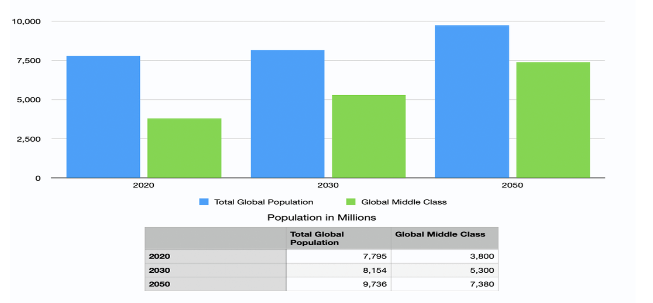
Figure 1: Growth of the Global middle class consumer
As the global middle class is forecast to approximately double over the following 30 years, global protein consumption is also set to double. That is a function of income. The growth of the middle class in these emerging countries will increasingly demand more fish, chicken, beef and pork. If protein consumption increases that much, grain production (animal feed), will also need to double in order to produce the protein.
One can look at the average food expenditure for many different nations, and it clearly shows the increase in demand as per capita GDP increases. This argument makes quite a bit of intuitive sense. The global middle class is defined as households that annually earn between $5,000 and $50,000. Currently, half the global population meet this income definition, but with the continued development of the emerging markets, 75% of a larger global population will be in that income strata. Throughout time, as families have increased household income, they have allocated a higher percentage of that income to food and specifically protein.
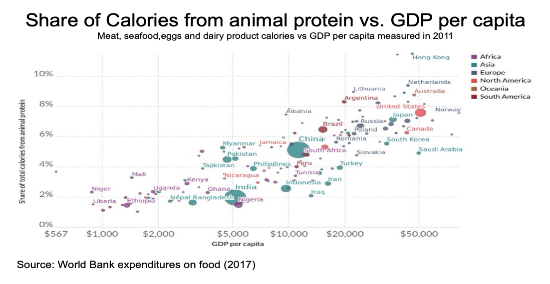
Figure 2
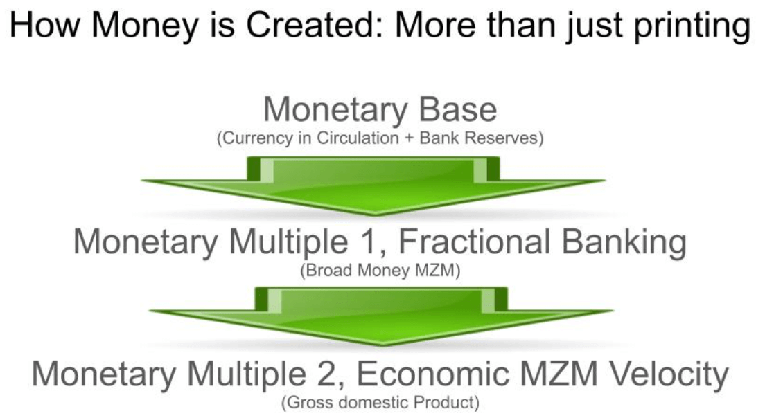
Second, if one considers the impact of inflation, farmland investing directly benefits from such an environment. The secret to understanding Inflation is understanding how money is created. It’s not just the amount of currency notes the Federal Reserve prints, it’s also about how that currency is multiplied in the banking system and the economy. Given the amount of currency created at the Federal Reserve during the past two economic downturns, it is now commonly believed this will eventually show up in increased inflation. I want to start to quantify how much potential for inflation is in the “pipeline”. If the banking system and the economy can return to the long term average multipliers within the banking system and economy, it would result in a 7 percent inflation rate compounded over the next 20 years.
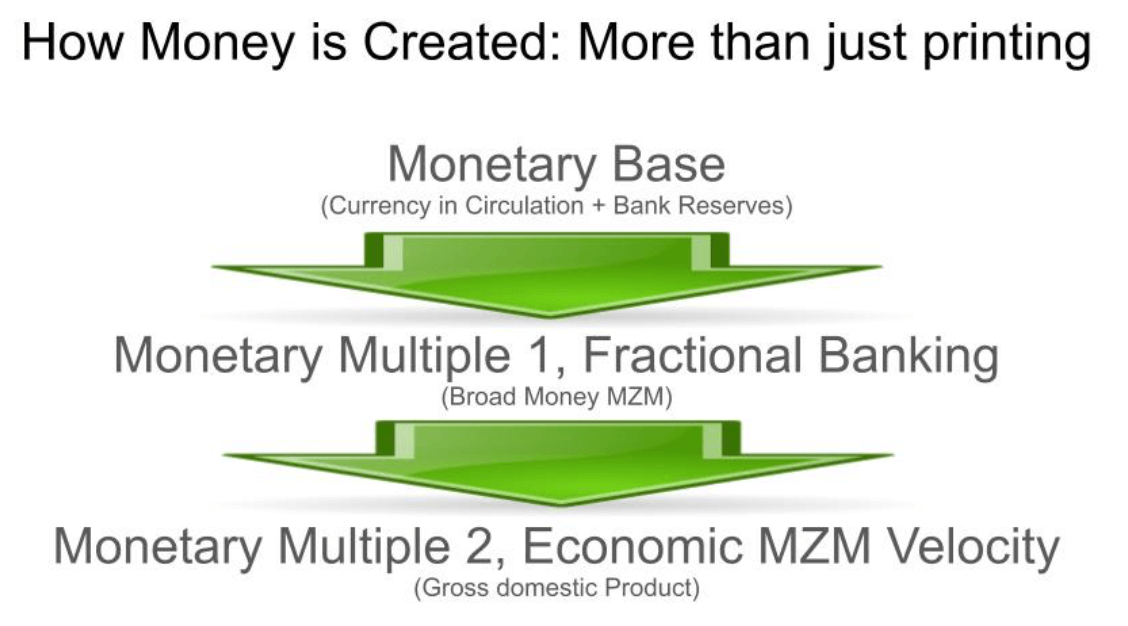
Figure 3
For example, in a quick review of fractional banking, if the Fed prints $1,000 and buys a bond. The $1,000 is deposited into a bank. This process is “multiplier 1” in the above table. The bank then takes a portion of that $1,000 and loans it out again. If the “reserve requirement” for that is 10 percent, then $900 will be loaned out and $100 will be kept back for “reserves” for the bad bank loans. Next, that $900 of new loans are deposited in other banks, and once again divided into $90 of reserves and $810 of loans. This process is repeated throughout the banking system if there is sufficient demand for loans. In total, the eventual total deposits created is 1 divided by the reserve requirement, or in this example 10, one divided by 10 percent. For every dollar the Federal Reserve prints, 10 dollars of deposits can be created in the economy.
Multiplier 1, the traditional ratio of broad money supply (MZM) to the monetary base, has averaged 8.52 from 1999 to 2007. But after the financial crisis of 2008, the banking system has been slowed to deal with increased regulation and increased money being placed into bank reserves, and lower interest rates. Currently, this multiplier of MZM/ Monetary base is at all time lows of 4.15. This means, if the effective bank money multiplier returns to the normal range, the total money supply in the banking system should approximately double, without the Federal Reserve even printing a single additional dollar.
What if the banking system multiplier returns to normal?
What is the potential inflation rate, given the money printing the Federal Reserve has done so far. What should MZM be if the economy was back to 1999 – 2007 normalities?
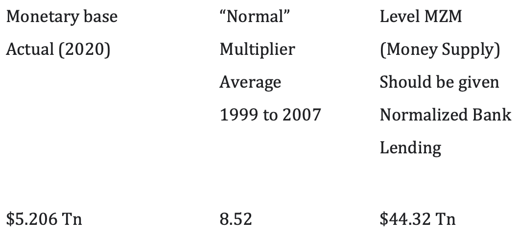
The Total Broad Money Supply (MZM) should be approximately $44.32 tn instead of the current 21.61tn, if the banking system returns to past activity.
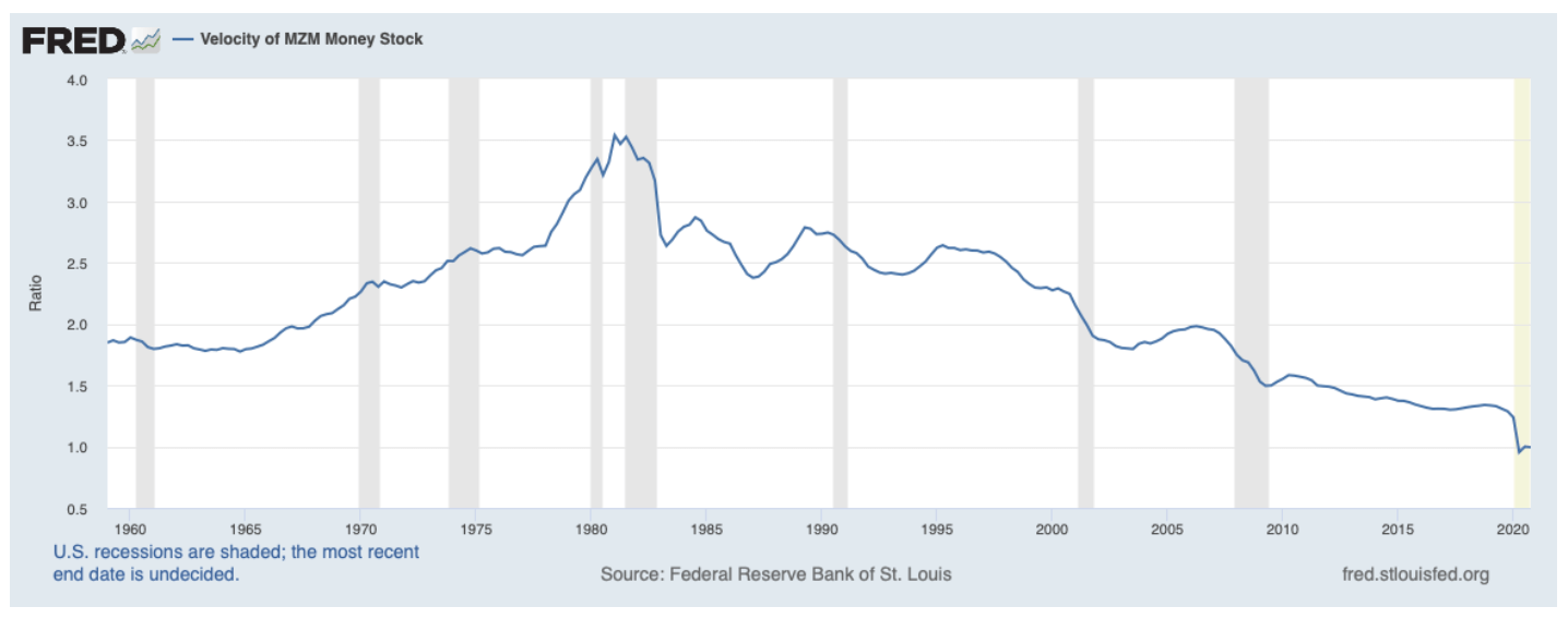
What if the MZM velocity in the economy returns to normal? This is the typical MZM velocity reported by the Federal Reserve.
Now, if we adjust the theoretical MZM, to what the nominal GDP should be under normal MZM velocity, then nominal GDP would be $85.09 Tn (Multiplier 2).
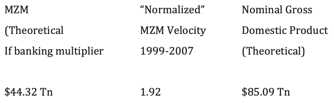
So, if the economy normalizes and returns to the average monetary ratios, for both measures, from the pre-crisis (1999 to 2007) level, then this current nominal GDP should be approximately $85 tn, instead of the current level of $21.479 tn. Because nominal GDP is made up of “Real (productive) GDP” plus inflation, I contend that the difference between the Theoretical GDP ($85 Tn) and the actual observed GDP ($21.479 Tn) is “Potential Inflation” of ($63.521 TN).
If the economic function returns to normal over say 20 years, price indices should rise by 85/21.479, or 3.96 times. If price levels need to inflate to four times the current level over the next 20 years, the inflation rate would need to average approximately 7 percent over these following 20 years.
The conduit that is different, the reason why inflation increases when it has been held at bay for decades, is the increased government spending through direct deficit payments to the lower economic classes in the US. With central banks printing money and are activities in capital markets, the velocity of the new money is very low. It primarily affects investment yield and risk curves, as well as increases banking system reserves. This type of quantitative easing is in fact deflationary as interest rates are moved lower.
When quantitative easing is mixed with increased stimulus spending by the government, the effect is inflationary. Stimulus and infrastructure spending has a much higher velocity. Government infrastructure spend increases the banking system multiplier. At the current low level of interest rates, this type of fiscal spending is the only viable public policy to move the economy toward full employment, traditional monetary policy is simply not an option. This adjustment will increase inflation, whereas in the past it has not been a problem.
Farmland performs very well in inflationary times. It is important to realize that farming is going under some of the most profound changes we have seen in over 50 years. Technology is aiding farmers to both increase yields, and scale farms to much larger in size. A modern row crop farm (Grain) is at least 3,000 acres in size. If that land sells for around $6,000 per acre, then that’s $18 million in farmland that a farmer needs to use, before any equipment is bought.
Currently, this situation gives the farmer two choices; to either rent the land or borrow large sums to purchase land. If a farmer borrows too much money, they risk adding financial leverage onto an asset with large operating leverage. This is why renting large tracts of land is more attractive to a growing modern farmer, it keeps the farm balance sheet much healthier and lets the farmer concentrate on purely the production of crops. This transfer of farmland into the hands of long term investors is one of the most attractive investment opportunities of the 21st century.
Farmland investment has traditionally had higher returns with lower volatility, when examined over the past 50 years. Currently, investors who are eying the prospects of higher inflation, have been returning to the study of farmland as an asset class with its negative correlation and positive returns over equity or bond investments. The major problem that investors first recognize is that farmland is a complex asset to acquire, manage and sell. Traditionally the asset is locally owned, and of course locally worked. These traditional difficulties are now changing.
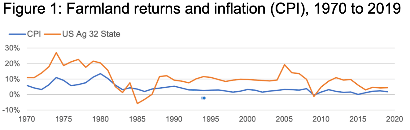
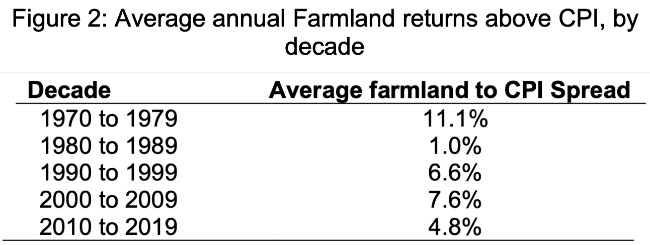
Given the investment climate introduced above, it seems timely to explore the relationship between farmland investments and inflation. Understanding the relationship between inflation and farmland returns, through a historical lens, gives an important roadmap to making money in the future. Farmland is a large asset class with about $3 trillion in aggregate value as of 2020, (USDA). During the past 50 years, farmland has consistently outperformed the CPI (consumer price index). This feature sets it apart as a unique asset class. We can also look at the average annual farmland returns ABOVE the rate of inflation CPI, over the past 50 years. Below is a chart of these returns grouped by decade.
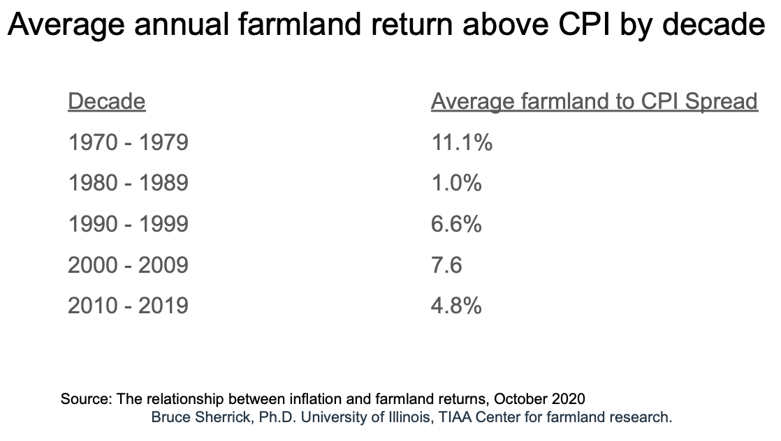
Figure 3: Average annual farmland returns above CPI by decade
The decade that jumps out at you is the decade of the 1970’s. During that time farmland returned 11.1% over the rate of inflation (USDA). This outperformance over inflation is primarily because during inflationary cycles, commodities tend to be inputs and generally finished goods manufacturers have difficulty keeping up with pricing pressures and margins decline. The net effect is that raw materials often show stronger rates of inflation above the consumer price index. Also, as commodity prices rise, the productive capacity to produce those commodities (such as farmland) tends to increase in economic value even faster than the commodity price. In addition, farmland is becoming more productive with more grain being produced off of a given amount of acreage. Therefore, farmland has shown much better returns than just the commodity. With the increased use of technology, this productivity increase looks set to continue.
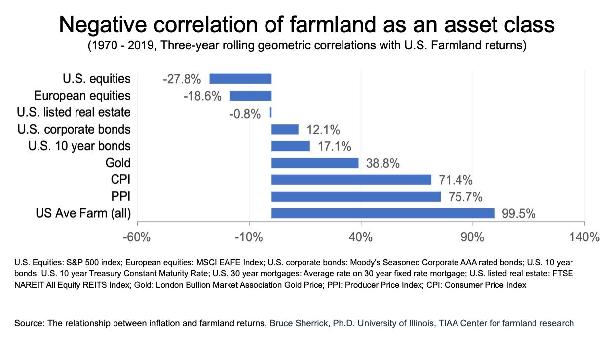
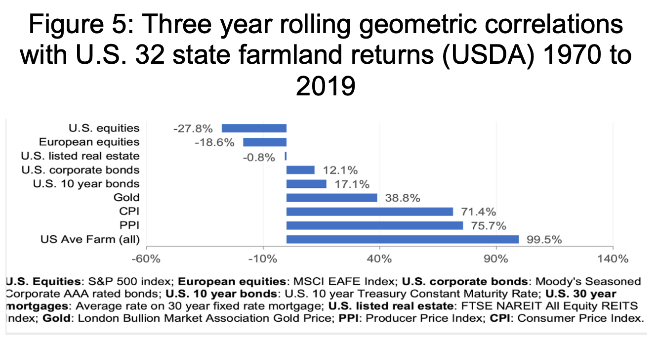
Most importantly, the returns for farmland has a high negative correlation to equities, and low correlation with bonds. If you believe we are headed for higher interest rates, then farmland provides an asset class that should benefit from such an environment. Gold is also a popular inflation hedge, but looking at the statistics over the past 50 years, it has significantly higher volatility. Gold doesn’t provide any income, and tends to outperform only when inflation expectations are increasing. Farmland returns tend to be more stable over CPI, even when inflation expectations are stable and moderate. In stable moderate inflationary times, investors seem to be bored with gold and it tends to have negative years, while you still get a crop and positive returns on a farmland investment.
If one looks at total annual returns for farmland, over the past 50 years farmland has had superior returns, performing better than equities, bonds, or gold. Equally as important, the volatility of the returns is lower than equities or Gold. The coefficient of variation is the standard deviation of annual returns (Volatility), divided by the average annual return of each asset class. So it gives an investor a measure of how much volatility they must experience for each unit of return. The lower the Coefficient of variation, the better. Farmland as an asset class has both higher return and lower volatility than equities, and in relative terms the volatility to return ratio is 3.5 times higher for US equities vs US farmland. The chart below was calculated from a University of Iowa agricultural professor. He calculated the total return for farmland investment in the 32 largest agricultural states over the past 50 years. From the raw USDA data, he could measure both annual return and volatility.
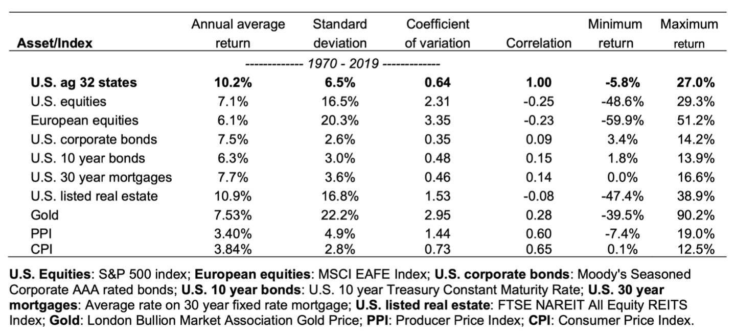
Figure 5: Volatility and long term returns of farmland investing
As examined in this introduction, as inflation increases, farmland returns tend to outperform the level of CPI. During the 1970, farmland returns averaged 11.1% above the level of CPI. If we are conservative and assume only half this level of outperformance happens in this next inflation cycle over an estimated 20 years, farmland should appreciate approximately 5.5% above inflation. We estimate a conservative future rate of inflation to average at least 7 percent per annum over the next 20 years. This would be the rate of inflation if monetary multiples return to pre Global Financial Crisis levels of 2000- 2008, not the higher rates of the late 20th century.
When added together this indicates that farmland could provide a nominal returns of 12.5% per annum over the following 20 years, or more. Once again, I think these are conservative estimates, and the risk to my forecast is that inflation has a higher average than I estimate. Afterall, the UK in the 1970’s averaged 13.8% CPI inflation. Given our debt and increase in the monetary base exceeds the UK’s heading into this period, the risk is on the upside. On the following page there is a graph showing the total return of an investment at 12.5% compounded for 20 years.
In this type of inflationary environment, bonds would get hit quite hard as rates increased. Equity valuations would roughly half, so earnings would need to double just to keep your investment at whole. Furthermore, corporate margins suffer during inflation because of inability to pass along cost increases. Put together, we believe that farmland represents a new institutional asset class that is set to outperform other asset classes strongly over the coming decades.
The Case for Agriculture 2050
Farmland has one of the highest potential returns for investors going forward. Although it has been traditionally difficult, as a passive investor, to participate in this sector of the economy, this is changing. There’s a strong fundamental case for the increased demand for food, as well as supply issues going forward.
The case for farmland investment breaks down into five key drivers of demand. Going forward, I believe farmland investing is the most levered play to the continued growth and development of the global economy.
- First, although at a slower overall rate of growth, the global population is still growing strongly. By most estimates, the global population should grow from the current 7.7 billion to 10 billion people by 2050. A slowing of the rate of growth from the 1960’s and 1970’s, but still very positive.
- Second, the overall population is continuing to industrialize, and a higher percentage of the global population will enter the global middle class (5,000 USD per year/ per household and above). This group is estimated to double by 2050.
- Third, once a family joins the global middle class, their basic needs of shelter and heat are generally, met and they tend to spend a higher amount of their income on protein. Their diet tends to bring in more beef, chicken, and pork.
- Fourth, given these drivers, global protein consumption is set to double by 2050.
- Fifth, if global protein consumption is going to double, then grain production must double as well. Grain is the main feed for chicken, hogs, fish, and cattle.
With grain as the primary input for protein creation. Given this global increase in demand, a few other investment attributes seem to rise to the top.
- US and Brazil are the only major block of agricultural lands that can create this supply and satisfy new global demands.
- Smaller farms in Asia will turn more toward fruit and vegetable production which is much more labor intense. Their industry is simply not set up for large scale, modern, and efficient grain production.
- Investments in this production chain are highly leveraged to the growth in demand. Farming has always been a business with great operational leverage.
- Given the new environment of very low interest rates and extraordinary monetary policy, farmland also benefits greatly from inflation. Through both debt and inflation, farmland also offers some of the greatest inflation leverage as well.
- Agricultural tech is also a way to invest in this process. Larger amounts of seed genetics and “precision farming” techniques will be needed to increase grain supply. With the average size of Chinese or Indian farms at approximately 2 acres, they simply cannot absorb new technologies that would increase grain production, and government cannot displace these farmers without significant social unrest.
Demand is increasing for agricultural products
There are two main drivers to the demand growth for agriculture, the first is simply the increasing population of the planet, and the second investment driver is the increasing calorie and protein consumed per person. Clearly, the number of mouths to feed is going up, and as the planet is getting wealthier, there is more demand for meat and protein. This situation provides opportunity.
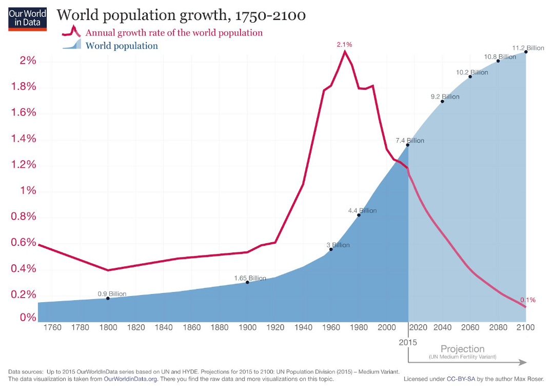
It is especially interesting to note that this increase in population is not dependent on a higher birth rate, in fact it assumes birth rates will fall sharply. The chief component of population increase going forward are improvements in medical care, diets, and standard of living which lead to longer lives. Not only is the population increasing, but it’s getting relatively older. Even with assuming a sharp drop in birth rates, in absolute terms the global population is expected to grow approximately 30% higher than the current global population by 2050.
As industrialization of the developing world continues, so will protein consumption. This has been widely observed throughout several cultures. Once minimum needs are met for shelter and clothing, then meat consumption increases. If an additional 3 bn people enter the global middle class as expected, the global demand for protein should double.
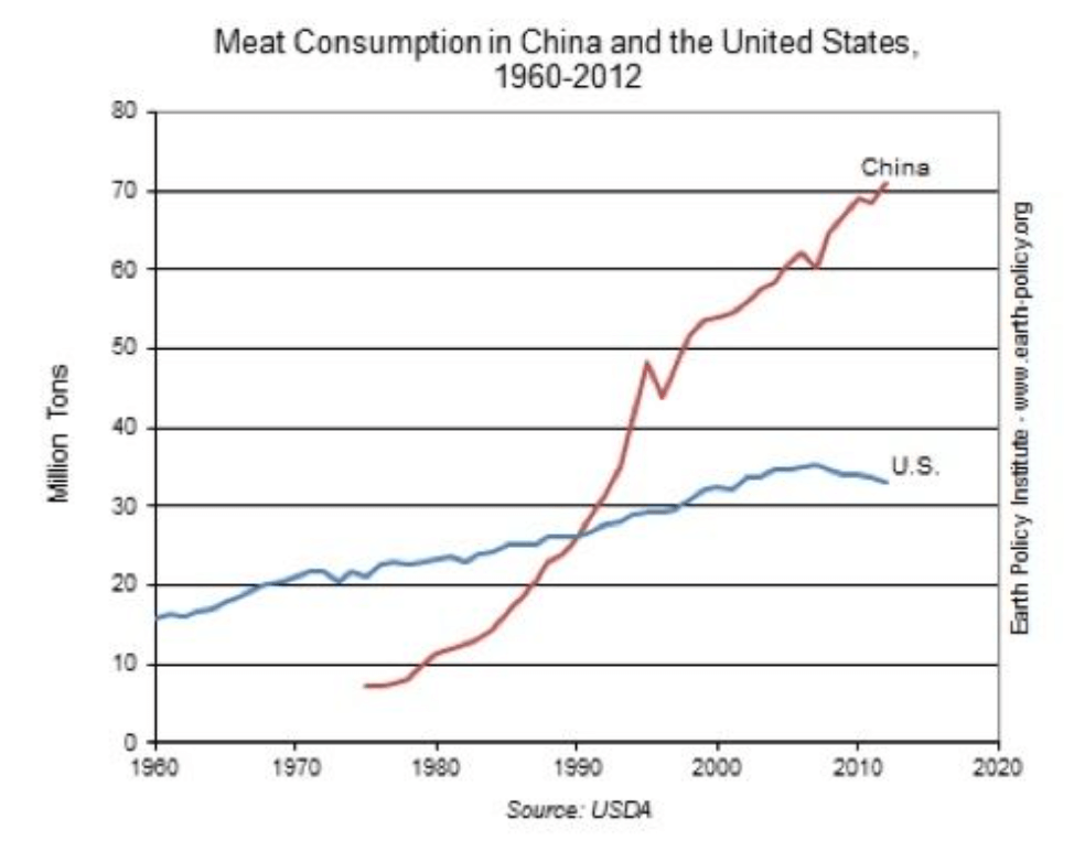
The global middle class is defined as households that make over $5,000 per year. Currently, of the 7 billion people on the planet, half of the global population is currently at or above the middleclass category. As incomes rise, it becomes more attractive for an individual or family to increase the quality and protein content of their diet. Below is a graph showing just how that evolved in China, in absolute terms. China’s population is much larger than that in the US, their per capita meat consumption is currently approximately half the US level, but in absolute terms total meat consumption is more than twice that in the US.
China still has a large percentage of their population in poverty, as development and incomes rise, even their consumption is still expected to more than double in the next 30 years. This story has played out in country after country, wealthier individuals consume more protein.
Increases in future grain production should come primarily from The US and Brazil, and therefore most of the investment opportunity going forward is concentrated in those two countries.
One other data set to look at is how much food expenditures increase as GDP increases. One can get a sense of where different regions and countries are going through looking at a graph of where all countries fall on this comparison. Below is a chart that shows a very linear and increasing relationship between amount spent on food and per capita GDP.
Note that annual food expenditure in Hong Kong is quite high. There are a few reasons for this. It is generally harder and more expensive to supply an individual Island like Hong Kong, but also in a very urban setting, people tend to spend their money more on food. I also think the Hong Kong example shows culturally where China could go. Although China spends a lot on food, they have a lot of people. The Hong Kong example does show an indication that China as a whole, could eventually consume somewhere in between Singapore and Hong Kong as food expenditures grow. That is still a lot of growth to look forward to.
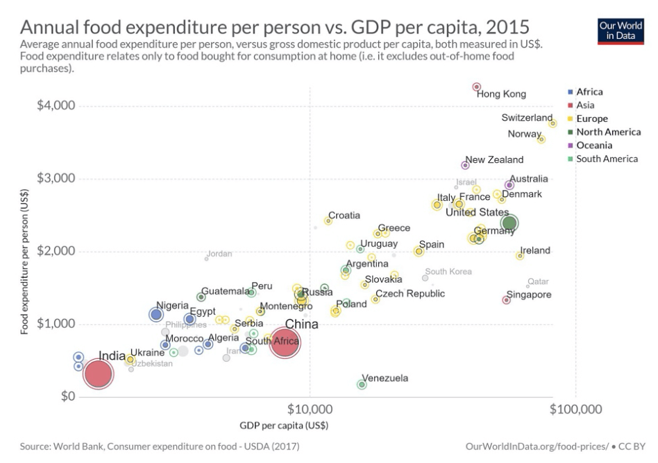
India also is the waking giant. It is true that India consumes less meat per capita than other developing countries, but this chart shows it still has a wide margin to increase it spends, as it continues to develop. It may not be as much into consumable meat, but they will still increase consumption of protein, perhaps more plant-based, and this will still increase demand for grain. Even if the entire world gave up meat consumption, it would generally cause a reduction in rangeland use, but the same acre of grain producing land would still be needed. Either by substituting higher priced crops that are generally picked by hand, or increased consumption of plant-based proteins. Both still supplies a lot of increased demand for agricultural goods.
So, what are expectations for middle class growth, and how does one quantify how much of an increase in protein is expected. From looking at world population growth, the world is approximately 7.6 billion people right now, and is expected to reach 10 billion by 2050. Furthermore, the global middle class is currently about 50% of the population, or roughly 3.8 billion consumers. If industrialization keeps growing as it has, the middle class (above 5,000 USD per year income) should increase to be about 85% of the global population by 2050, or 8 and a half billion people. We think this estimate is a likely figure over the next 30 Years. After all, over the last 30 years the middle class has essentially quadrupled, so actually just doubling over the next 30 years is a slower rate of growth than in the past.
Given past increases in middle class development, in many different countries, given the historic relationship of protein consumption and wealth, one would therefore expect global protein consumption to also double from approximately 200 million tons to over 400 million tons by 2050. Assuming global demand moves more towards a mixture of chicken and pork and even excluding beef production, that would indicate that global grain demand could rise from 1100 million metric tons of corn to 2200 m metric tons. Perhaps farmed fish diets go up, while demand for beef generally might fall, but overall grain demand still needs to go up irrespective of the diet mix at an alarming rate. Who can double grain production in the next 30 years? This task most likely falls on the US, Brazil, and potentially Russia, as the other countries most likely focus on higher valued vegetables and fruits. Each country faces its own strengths and weaknesses.
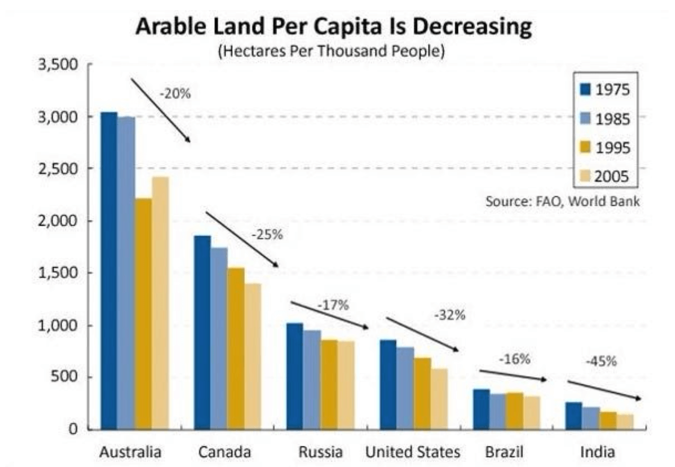
Global agriculture is also facing supply risks. At every farm sale I would go to as a little kid, the auctioneer would always point out “that they can’t make land”. If you look at farmable land on a per-capita basis, the availability of farmable land, per mouth to feed, has fallen in every major region of the globe. Below is a graph showing the change in arable land by region. It is especially interesting to realize that even in a country like Brazil, where they have brought into production vast areas of the Amazon region over the last several decades, total farmable land per capita is still falling behind. The population is has simply grown faster.
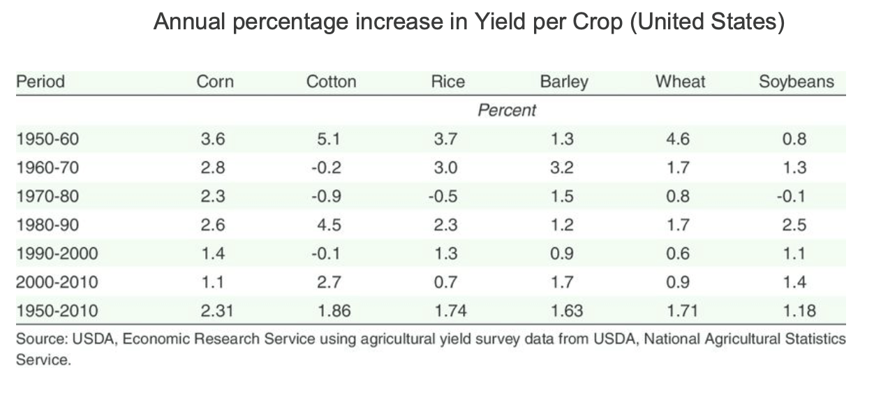
The relative decrease in farmable land has been made up through increases in productivity of the smaller amounts of land. The future danger is, that productivity increases have shown signs of decelerating. Decade by decade, since the 1960’s, increasing yields have become harder to find. Corn, Rice, and Wheat have all shown decreased growth in yields. Soybeans have demonstrated a lower but at least stable increase in yields. Still only averaging 1.18 percent per year since 1950. This low yield growth cannot generate a doubling of production over the next 30 years.
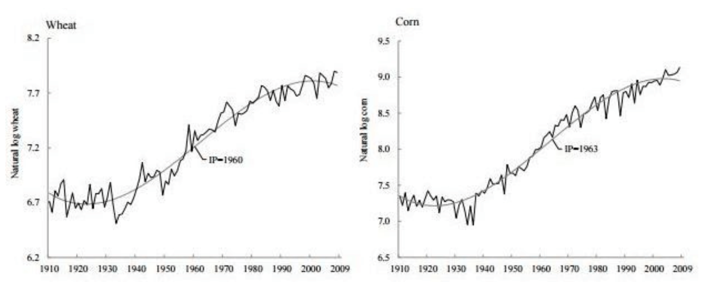
Researchers at UC Davis have been looking into falling agricultural productivity in developed countries. Their research points to a peak in productivity growth in 1960 for wheat and 1963 for Corn. The same data is there for soybeans, although soybeans were introduced later and therefore their peak in productivity yields happened in the mid 1970’s. These figures reflect the peaking of hybrid genetics on the farm, as farmers adopted higher yielding hybrid plants. As any innovation is introduced, and applied, there is a pick-up in productivity, followed by a slowing, as the innovation becomes the status quo.
Why does the US have a competitive advantage?
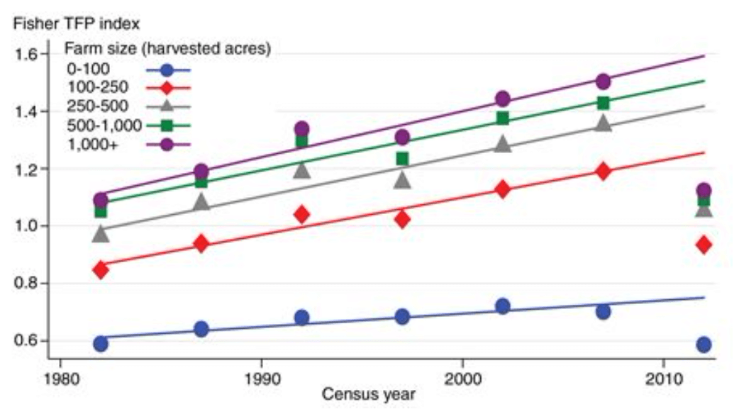
It is important to establish the impact of farm size on productivity. If one looks at the productivity of different farms based on farm size since 1980, one can see but the larger arms above 250 Acres are able to invest in capital equipment and therefore benefit from new technologies. The problem is when you see farms under that 200-acre Mark, they simply don’t make enough money to allow for any kind of R&D investment, therefore they fall farther and farther behind.
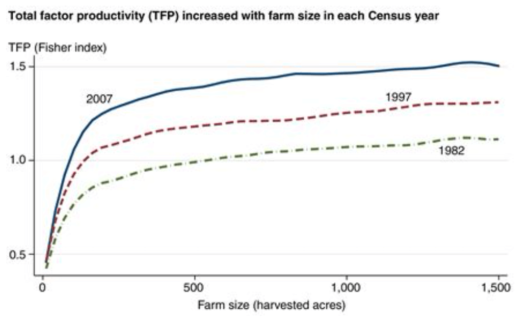
In the next graph, one can see the effect on productivity and size more clearly with each farm census year. When you can see Fisher’s Total Factor Productivity index, that’s the ratio of outputs over inputs, increases dramatically at about the 200-acre mark.
This relationship makes intuitive sense because for decades you seen how larger farmers are able to get larger, and that’s because their productivity is also higher, because innovation costs can be spread out over more acres. After all, if you’re buying a new drone to be able to take infrared pictures of your crop and detect weeds and drought, it makes more sense to spread those fixed costs over the 2,000 acres rather than just a hundred. The cost benefit of new technology is much more attractive for the larger Farm.
The impact of farm size becomes apparent as you begin to look at agriculture on a global basis. The average farm size in France is around only a hundred acres; the bread basket of Western Europe with the largest production of agricultural Goods in the EU. Even more striking is the average farm for the entire European Union is below 20 hectares, or about 50 acres. Having farms this small makes it very hard for those farmers to adopt new technology, it keeps their productivity relatively low. That’s why a large portion of the EU budget is spent on Farm subsidies.
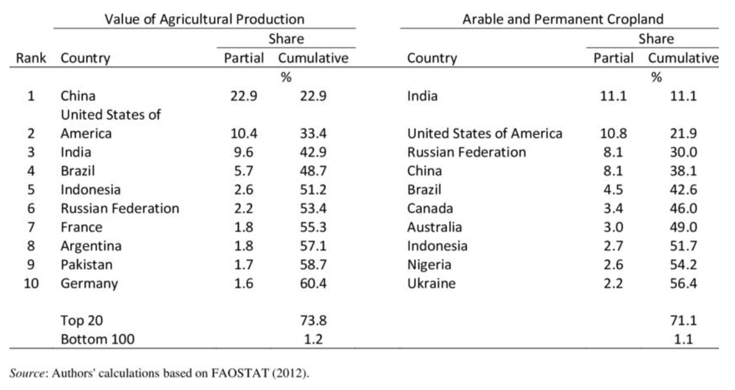
So how does the global production and available land break down?
If you look at the two columns in the following table, the first column on the left is the value of agricultural goods produced per country, and the second column on the right is the percentage of farmable cropland. One thing that jumps out at me is China’s placement. By far, it is the largest producer of agricultural goods, and they do it with only 8% of the arable land.
If you look into the figures, it is because they use one agricultural worker for on average every two and a half acres of land in their country. In essence they’ve been able to increase their farm output by intensively farming their existing farms with more people.
The only problem is where do they go from now, how to increase production? Since China already intensively farms with a large number of laborers, it also means that they will not gain much through mechanization. Their labor force already produces with great care and attention, producing as much as the land can produce, but modernization will not bring them much more. This means the world has to look someplace else.
While during most years, China’s agricultural production is sufficient to feed itself, in drought years, China must import more grain. Due to the shortage of available farmland, and an abundance of labor, it makes more economic sense to import land-extensive crops (such as wheat, rice, corn, and soybeans) and to save China’s scarce cropland for high-value and labor-intensive crops, such as fruits, nuts, or vegetables.
Since the revolution in the 1950’s, in order to maintain China’s grain independence and ensure food security, the Chinese government has enforced policies that encourage grain production at the expense of more-profitable crops. This is changing. In 2015, the Chinese government eliminated price supports for very small corn producers. This resulted in lower prices as government inventories were liquidated. But now corn prices are hitting new highs in China. In 2018, for the first time in 7 years, China’s corn crop was unable to meet its domestic demand. Even with this reform, corn prices in China are over 7.25 US dollars per bushel, in contrast to the world price of 4 dollars a bushel.
For policy makers in India and China, the priority 50 years ago was independence. Now that they are industrially developing, their priority is becoming efficiency. The difficulty in increasing efficiency is keeping economic and social order. Currently farms are farmed by individuals with very little education and their small plot of land is rented from the collective. Simply put, the priority in countries like China and India, have been to primarily focus on industrial production in manufacturing increases. Agriculture was seen as a way to keep lower class citizens employed. If they start to merge farms into much larger modern farms, the social unrest from large numbers of unemployed farmers would be untenable for these rapidly changing societies. They will most like place an increased emphasis away from grains toward fruits and vegetables.
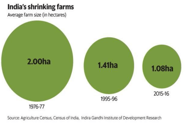
India is another case, although it has the highest farmable land acreage on the planet, its productivity has been limited. An ongoing issue with India has been the shrinking size of their average farm. As populations have grown, there have generally been multiple inheritors of a farm which then divided up that farm to even smaller plots. Both of these issues are well-known in both the Chinese and Indian governments, and over time they need to be dealt with, but it will take several generations, not just 30 years, to get their agricultural production up to Modern productivity.
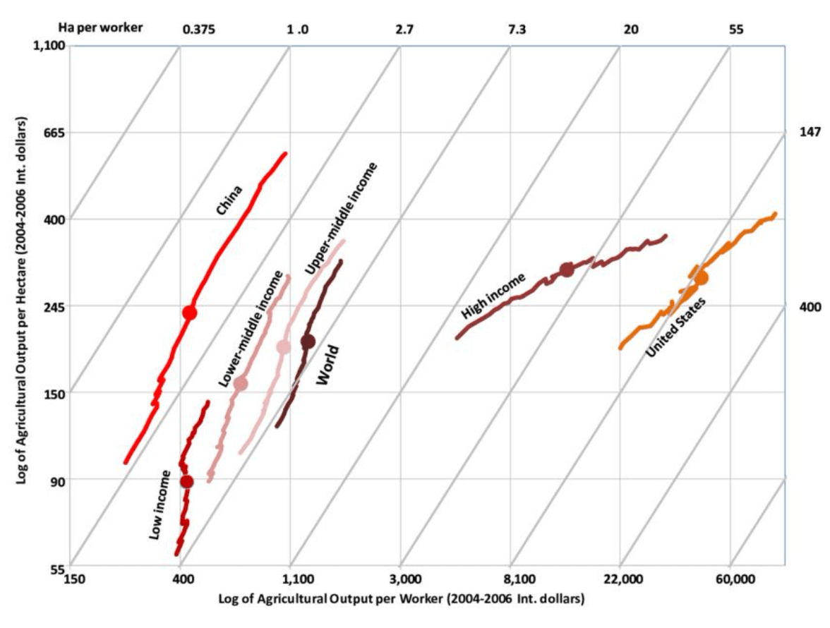
The final change graph is a summation of the history of global agriculture since 1960. It’s a little difficult to understand, because it’s a graph that is graphed on three axes. In general, the graph is graphing the value of agricultural output per acre, as well as the agricultural output per worker for each country through time. You can see as each region evolves and how the different characteristics of that region are playing out.
First look at the far-left line of China. They started off with very low productivity per hectare as well as low output per worker in1960. Through various central planning arrangements, they were able to actually use more workers per acre and dramatically increase the output per acre up to Western standards. This is primarily through the very intensive individual laborers and higher valued vegetable, nut, and fruit production. But where does production growth go from here? I think Chinese agricultural production will move toward more “truck” farming and away from grain production.
We can also see a different trend in the second to the far-right line of high-income countries. These countries like the UK, France and Japan. These countries have seen a rapid increase in the number of hectors farmed by each laborer, but from what we know of farm size their productivity, still is not quite where the US is.
Finally, on the far right, you can see the US developed to now 200 hectares or 440 acres per laborer. Because of the larger farm size, the US is able to adopt new farm technology at a faster pace, and this is good for production.
This chart captures the competitive environment of all of the regions and types of farms on the globe. We’ve gone through the challenges and advantages that countries like China and India have, if they are to increase production. Next, we look to the competitive advantages that the US has in further increasing the agricultural sector value chain, and finally the challenges the world faces with the slowdown in yield growth.
US geographic advantages
First, the US offers geography. They have the largest cropland mass in the world located in latitudes that are favorable to crop production. The US is also midway between the export markets of Europe and Asia. Internal geography gives the US the largest internal river transport network. The Mississippi, Ohio, and Columbia Rivers, can transport large amounts of agricultural goods at a very cheap price compared to other competitors. Infrastructure like Port facilities, rails and highways, as well as the elevator and storage systems for grain, are much more developed than what we see in other countries like Russia or across Europe.
When you consider technology and capital used in agriculture, the US has a large competitive advantage as well. The new agricultural Innovations that industry is developing in the economy are largely based on artificial intelligence with autonomous vehicles. Research and development in the US are in the global leadership position.
The US also has a great system of land grant colleges. This is something that’s unique in the world. As a society, the US has chosen to have one of the highest educated labor forces in agriculture in the world. It is these college-educated farmers that can understand the new technology and apply it in a judicious and productive way. US farms are also well-capitalized. An average farm size of 440 Acres generally provides a lot of family equity to the business, which can be used to educate the next generation of farmers and keep productivity gains high.
So, what does all this mean? The total global population is most likely to grow to 10 billion people in the next 30 Years. The movement globally to industrialize and increase per capita GDP will probably continue. Sure, certain individual countries might experience more problems than others, but the general march of industrialization continues. With industrialization, global wealth will also rise and demands for more and better food will increase.
Inflation is the kicker
The case for investing in agricultural farmland is also a major beneficiary as inflation increases going forward. First, inflation, which has been generally falling since 1980, will tend to move higher over the coming decades. Although global inflation is not required for the base agricultural thesis, it sure does turbo charge returns and we think its return is quite probable.
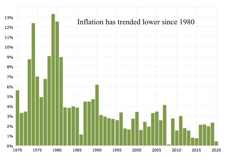
During the decade of the 1960’s and 70’s, inflation rates across the globe increased sharply. But once inflation rates peaked around 1980, investors could get used to the idea that the value of their currency would remain more stable in the future and they would not face inflationary depreciation going forward. This change in inflation expectation, allowed Bond markets to rally strongly as interest rates fell, and bond prices therefore increased. Below is a chart of the US Treasury 10-year bond, which peaked at a 16% yield, and currently has fallen to less than 1%.
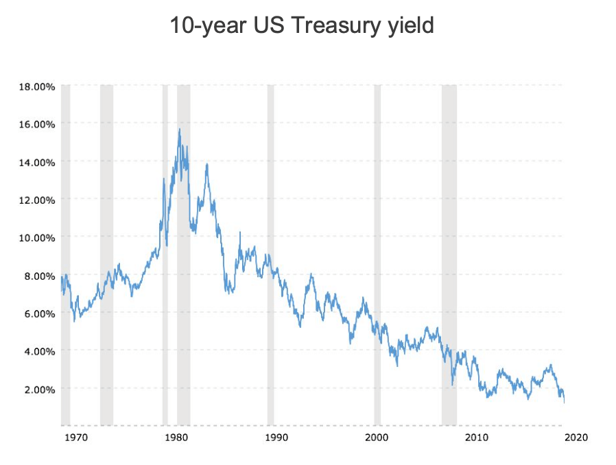
This general fall in the cost of money from 1980 through 2020 created a distinctly different investment condition than what exists now. Mathematically, the cost of money or interest rates cannot fall in a similar way over the next 40 years. There is a zero limit for loans and credit. Yes, government bonds can technically move into negative rates, but the commercial side of debts cannot. When rates are negative, that means the entity making the loan agrees to in total to receive less money than the initial loan in repayment. While government bonds can be bid up to negative rates in panics. But in commerce, banks will simply not make new loans under the same situation. They will hold cash.
The fall in interest rates had a large impact on the economy. As the cost of money decreases, governments, corporations, and individuals borrow even more money without paying more in annual interest cost. This increases aggregate demand in the economy. Over the past four decades, this has been a great tool in helping to dampen the business cycle, central banks could lower rates in a recession, which would therefore create more demand and move the economy out of recession.
With interest rates at the zero bound, the only way to increase aggregate demand is fiscal spending. Deficits are set to explode, and now both parties seem to be in favor of this. When the Federal Reserve now asks for fiscal support, what they are asking for is that governments spend in deficit and put the money out into the economy to increase spending or aggregate demand. At all times in history this has been inflationary. This is not just quantitative easing, but full monetization and inflation of debt. There is plenty of debt to drive this inflation going forward. There is simply too much to actually pay off, so economies are now forced to inflate away the debt. This will take a lot of global inflation.
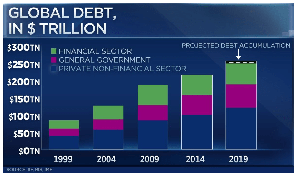
At no time in history has there been more debt in our country. Furthermore, our borrowing binge has extended into foreign borrowing as well over the last 20 years. Total Global debt has expanded to 288 trillion US dollars. 20 years ago, the value stood at just approximately 88 trillion US dollars. Most of the recent borrowing has come from the expansion of credit in China and the US, and these two countries have been lucky enough to primarily borrow in their own currency. If they ever really need to pay it back, all the Chinese or Americans needs to do, is print the currency.
This debt has been there for many years, and we’ve seen very few inflationary pressures. Why does inflation happen now?
Inflation comes from the regular cycle we have witness many times before. Financial assets move forward, and eventually leverage increases, and the pressure to inflate becomes the only politically acceptable way forward. Real Assets then start to outperform as interest rates and inflation rise. With several of the global 10-year government bonds yielding a negative return, and the US 10-year treasury yield around .8%, there’s simply not the room, or the math, for the economy to move forward and aggregate economic demand to be regulated from the lowering of interest rates.
Fiscal policy is therefore increasingly important moving forward. Future recessions will be fought primarily with government spending, not changes in interest rates. Wealth inequity is at historic highs, as it usually is near the end of financial booms. Money given to the lower half of income levels has a much higher propensity to be spent and therefore has a much higher velocity. The velocity of this redistribution is quite high compared to the first rounds of quantitative easing. Government guaranteed loan programs, like the PPP, also increase the multiplier through the fractional banking system. This process both increases lending and spending, in an effort to avoid ever deepening recessions. That’s why deficits will probably increase from here, money will be directed toward spending and creating demand, and quantitative easing will keep printing money to fill the gaps. All taken together, this should be an environment less supportive to financial assets and tend to increase inflation.
So, in conclusion, this is the case for agricultural investing. The supply-demand balance is shifting to cause real prices for grain to go up, and secondly the financial situation of the globe means a high level of debt will most likely be controlled through inflation. During inflationary environments in the past, farms have performed very well.
Farmland investing is not fixed income
In the past farmland has been sometimes thought of as a surrogate to fixed income. Many potential investors ask me what is the current yield on farmland. I believe some major differences need to be explained. It is, in many ways, an “anti” bond investment. Let me explain. You want to invest in farmland when inflation is increasing, and bonds fall in time of inflation. But as an exercise, let’s look at the numbers.
You want to buy farmland when the industry is a time period of stress. This means farmland tends to be cheaper when current yields are low. Historically, farm rental yields have averaged between 3 and 5 percent of current land values. Historically, you want to buy land when the industry is down, the rent income improves as the industry rises. In this way it is opposite to a bond.
A bond has a fixed coupon payment, and when the yield is low, that means the value of the bond is relatively high and in danger of creating a capital loss as rates increase. The opposite is true with farmland. When farmland yields are low, crop prices are down. Values are generally down as well. As the cyclicality of the industry improves, the rental payment increases, and land values go up. For farms, low yield can indicate low valuation. For bonds, low yields indicate high valuation.
Let’s look at an example. Over the long term, farmland rental income tends to average approximately 4 percent of the land value. Let’s be conservative and assume a 3% rental rate. Remember, as discussed in our white paper Farmland as an asset class, we showed that historically farmland values have tended to increase more than inflation over time. In that white paper, we also forecast a total return profile, given expected inflation rates, of 12.5% returns for farmland.
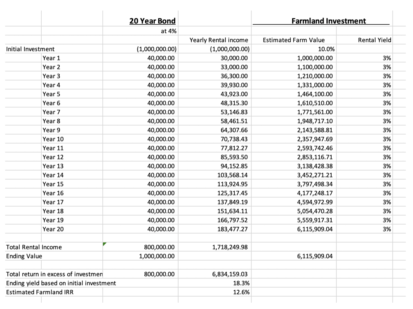
What does that look like? Below we constructed an excel sheet to illustrate the different returns streams of a bond investment and a farmland investment over a hypothetical 20 years. In this example, a million dollars is invested in both a 20 year bond and a farm. Notice that the beginning yield on the bond is above the farmland. By definition, a bond return is fixed, and farm income benefits from inflation while bond values decline as inflation increases. Note that we assume a 3% yield on the farmland based on the current market value of the land. Given a 3% farmland yield, then the underlying farmland value should increase at approximately 10 percent if inflation is at 7%.
Of course as in any pro forma, the returns will not be this even. In reality inflation will start off slower than the average and then increase above the long term average, so the year to year changes will not show this even increase reflecting a 7% inflation rate. This is purely an example to illustrate an average farmland return if inflation averages 7% and farmland returns average similar levels over CPI as they did over the past 50 years. An actual farm return will be more variable, but this is designed to illustrate the average move over a two decade holding period. Once again please see the white paper Farmland as an asset class to see how we estimated these values. One nice attribute of farmland investing is that the yearly income grows overtime. In our example, the yearly income at year 20 represents a yearly yield of over 18% on the initial farm investment.
Comparison of Hypothetical Farmland cash flows vs Bond cash flows
Once again, the point of this example is to illustrate how farmland investment is a completely different asset class from equity, bond or even commercial real estate investments. As inflation and interest rates rise, the economics of farmland is very different, and creates unique returns as illustrated above. Commercial real estate is priced off capitalization rates, when capitalization rates increase with inflation, values decline. With inflation returning, remodeling and maintenance costs increase with inflation. In order to keep up with the replacement of depreciation, commercial real estate becomes increasingly expensive to keep up with. Farmland does not depreciate. If you keep improving soil health, it actually becomes more valuable. Bonds fall in value with inflation, and the yearly coupon return is fixed, farmland can increase its yearly earnings with inflation. Finally, equities have difficulties with inflation because valuation levels contract with higher interest rates, and margins for many corporations fall during times of inflation. Raw material costs are historically difficult to pass along.
Farmland as an asset class
It is important to realize that farming is going under some of the most profound changes we have seen in over 50 years. With the global middle class set to double by 2050, protein demand should also double. Technology is aiding farmers to both increase yields, and scale farms to a much larger size. A modern row crop farm (grain farm) is at least 3,000 acres in size. If that land sells for around $6,000 per acre, then that’s an $18 million farmland asset that the farmer needs before any equipment is bought. Currently, this situation gives the farmer two choices; to either rent the land or borrow large sums to purchase land. If a farmer borrows too much money, they risk adding financial leverage onto an asset with large operating leverage. This is why renting large tracts of land is more attractive to a growing modern farmer, it keeps the farm balance sheet much healthier and lets the farmer concentrate on purely the production of crops. This transfer of farmland into the hands of long term investors, and then renting it to farmers, we believe is one of the most attractive investment opportunities of the 21st century.
As an asset class, farmland investing has traditionally had higher returns with lower volatility, when examined over the past 50 years. (source) Currently, investors who are eying the prospects of higher inflation, have been returning to the study of farmland as a unique investment. The major problem that investors first recognise is that farmland is a complex asset to acquire, manage and sell. Traditionally the asset is locally owned, and of course locally worked. These traditional difficulties are now changing.
Farmland as a financial asset exhibits returns that are positively correlated with inflation. As inflation increases, farm revenues and total value generally increase. Farmland has shown a low or negative correlation with equities, chiefly because inflation benefits farmland while hurts equity investments, due to equity valuation contraction as interest rates move up. The volatility of farmland is also traditionally lower because of the relative lack of movement to short-term market news. Farmland is historically not hotly traded, relatively easily valued with over $3 trillion of comparables just in the US, and therefore more stable. Farmland is relatively simple to value given historic yield characteristics, price received for crop grown, and relative movement of inputprices. Farmland is simply not subject to the daily price swings like equity markets. Over the past 50 years, farmland has shown one third the annual volatility of equity, one quarter the volatility of Gold, and less than half the volatility of US listed real estate.
Over the past decade, since the Global Financial Crisis, investors have witnessed massive dislocations as interest rates around the world have been forced lower and lower. Capital was needed to rebuild the banking system’s capital. These low interest rates, along with extreme Central Bank liquidity, have moved together to elevate equity markets well above most historic valuation measures.
This is not the case with farmland. Over the past decade agricultural markets have been disrupted by trade wars, the coronavirus shutdown, and a rising US dollar. During this mini farm recession, in response to ag-sector income pressures, the U.S. agricultural markets have been supported by federal support programs including Market Facilitation Program payments, as well as by indirect and direct payments from programs stemming from coronavirus related stimulus. Farmland, in our opinion, is arguably one of the most undervalued asset classes available.
Given the investment climate introduced above, it seems timely to explore the relationship between farmland investments and inflation. Understanding the relationship between inflation and farmland returns, through a historical lens, gives a roadmap to making money in the future. In periods of accelerating inflation, raw materials often show stronger rates of inflation above the general consumer price index. Also, as commodity prices rise, the productive capacity to produce those commodities tends to increase even faster. Farmland has become more productive with more grain being produced off of a given amount of acreage. Therefore, farmland has shown much better investment returns than just the commodity. With the increased use of technology, this productivity increase looks set to continue.
Farmland is a large asset class with about $3 trillion in aggregate value as of 2020, (USDA). During the past 50 years, farmland has consistently outperformed the CPI (consumer price index), This feature sets it apart as a unique asset class. In general, when inflation is accelerating, then most commodities get bid higher as well. Gold often races ahead at the beginning of an inflationary cycle, but farmland has the ability to produce agricultural commodities consistently and show more consistent annual returns above inflation and gold.
When you group returns by decade, one clearly sees that farmland returns were far ahead of CPI during the past inflationary cycle of the 1970’s. The 1980’s were highly impacted by the “farm crisis”, when the US dollar soared, and very high leverage led to a crisis in farm credit. The 1990’s and 2000’s were characterized by general stability while the decade beyond 2010 was driven by the first Asian commodity cycle.
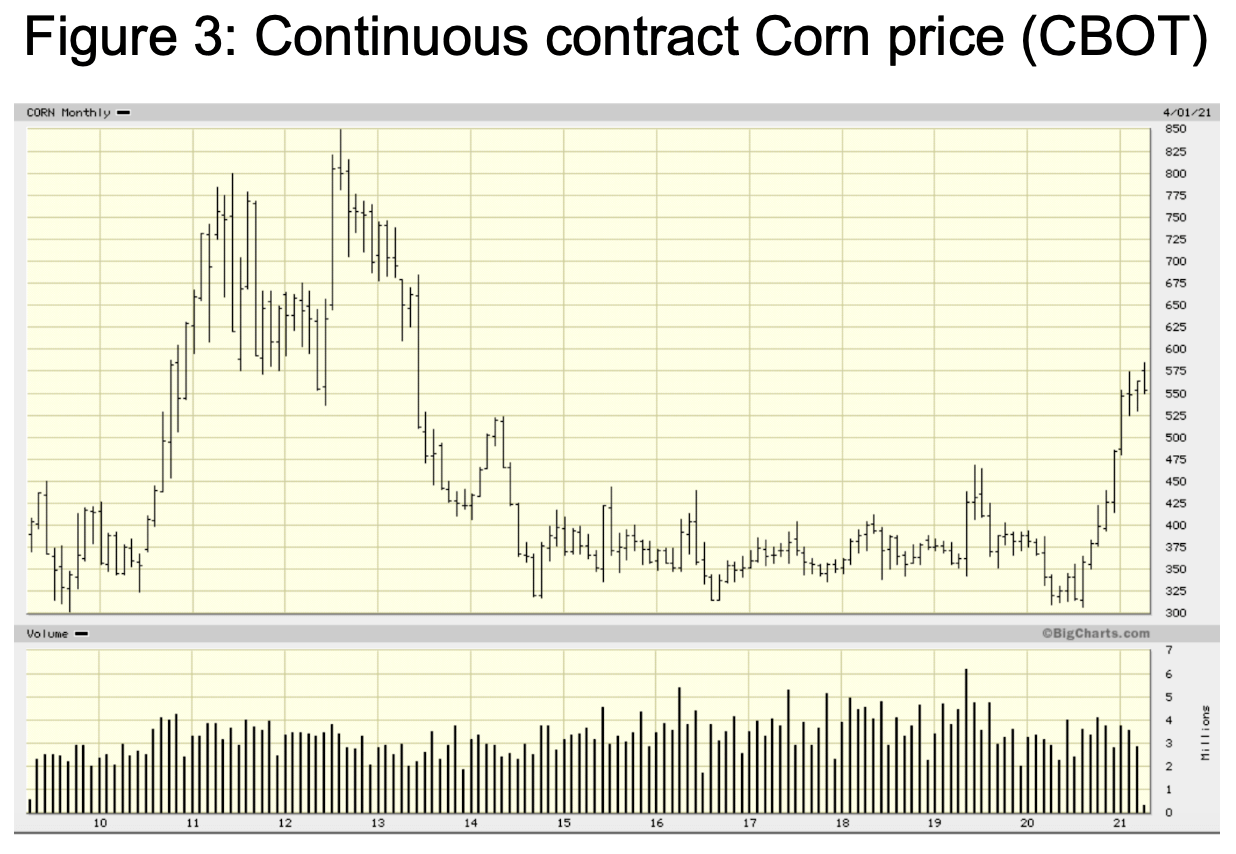
In the next chart one can see the strong rally in grain prices in the beginning of this decade. It is our belief that the next surge in agricultural prices will be driven not just by Chinese consumption, but a broader based increase in demand across the entire developing world. This broader based increase in demand should last over the next several decades as the global middle class begins to eat more protein, and the main feed for protein is grain. Simply put, the demand for grain is set to double over this same time period. Please refer to our white paper, The Case for Farmland Investment, for further details.
If one examines total long term annual returns for farmland, farmland has had superior returns, performing better than equities, bonds, or gold over the past 50 years. Equally as important, the volatility of the return is lower than equities or gold. The coefficient of variation is the standard deviation of annual returns (Volatility), divided by the average annual return of each asset class. So it gives an investor a measure of how much volatility they must experience for each unit of return. The lower the Coefficient of variation, the better. Farmland as an asset class has both higher return and lower volatility than equities, and in relative terms the volatility to return ratio is 3.5 times higher for US equities vs US farmland. The chart below was calculated from a University of Illinois agricultural professor. He calculated the total return for farmland investment in the 32 largest agricultural states over the past 50 years. From the raw USDA data, he could measure both return and volatility.
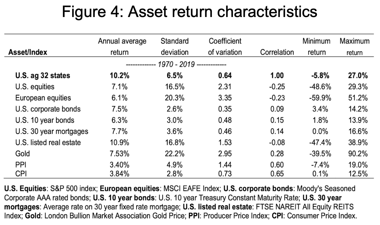
Most importantly, the returns for farmland has a high negative correlation to equities, and low correlation with bonds. If you believe we are headed for higher interest rates and inflation, then farmland provides an asset class that should benefit from such an environment. Gold is also a popular inflation hedge, but looking at the statistics over the past 50 years, it has significantly higher volatility and lower return. Gold doesn’t provide any income, and tends to outperform mostly when inflation expectations are increasing. Farmland returns tend to be more stable over CPI, even when inflation expectations are stable and moderate. In stable moderate inflationary times, investors seem to be bored with gold and it tends to have negative years, while you still get a crop and positive returns on a farmland investment.
We have examined the return characteristics of farmland over the past 50 years. But given what we learned, what does this tell us about future investments? If one considers an estimate for future inflation, we estimate this future rate given already incurred increases in the central bank’s balance sheets and a partial return to normal monetary velocities. We estimate a conservative future rate of inflation to average at least 7 percent per annum over the next 20 years. This would be the rate of inflation if MZM velocity only returns to pre Global Financial Crisis levels of 2000- 2008, not the higher rates of the late 20th century. For further details please see our white paper entitled How high do we think inflation would reach.
As examined in this paper, as inflation increases farmland tends to outperform even the level of CPI. During the 1970, farmland returns averaged 11.1% above the level of CPI. If we are conservative and assume only half this level of outperformance happens in this next inflation cycle over an estimated 20 years, farmland should appreciate approximately 5.5% above inflation. When added together this means that farmland could provide an average nominal return of 12.5% per annum over the following 20 years. Once again, I think these are conservative estimates, and the risk to my forecast is that inflation has a higher average than I estimate. Afterall, the UK in the 1970’s averaged 13.8% CPI inflation. Given the current US debt levels and increase in the monetary base exceeds the UK’s heading into the 70’s. The risk for our inflation forecast is on the upside.
In this type of inflationary environment, bonds would get hit quite hard as rates increased. Equity valuations would roughly half from current levels, so earnings would need to double just to keep your investment at whole. Furthermore, corporate margins suffer during inflation because of an inability to “pass along” cost increases. Put together, we believe that farmland represents a new institutional asset class that is set to outperform other asset classes strongly over the coming decades.
How high could inflation go
The secret to understanding Inflation is understanding how money is created. It’s not just the amount of currency notes the Federal Reserve prints, it’s also about how that currency is multiplied in the banking system and the economy. Given the amount of currency created at the Federal Reserve during the past two economic downturns, it is now commonly believed this will eventually show up in increased inflation. I want to start to quantify how much potential for inflation is in the “pipeline”. If the banking system and the economy can return to the long term average multipliers within the banking system and economy, we would be looking at a 10 percent inflation rate compounded over the next 20 years.
So the overall economic function looks something like this.
In the short run, these multipliers can be affected by regulation or productivity, but in the long term, they are very stable. So I would like to talk about a 20 year forecast for inflation. What would that look like? What does the long term history of these monetary aggregates tell us about the long term pressure on prices. This is not a perfect model, but it is robust in calculating a long term target for prices.
Function 1: Printed money multiplied in the Banking System
Fractional reserve banking is a banking system in which banks only hold a fraction of the money their customers’ deposit as reserves. This allows them to use the rest of it to make loans and thereby essentially create new money. This gives commercial banks the power to directly affect the money supply and create dollars.
For example, if the Fed prints $1,000 and buys a bond. The $1,000 is deposited into a bank. The bank then takes a portion of that $1,000 and loans it out again. If the “reserve requirement” for that is 10 percent, then $900 will be loaned out and $100 will be kept back for “reserves” for the bad bank loans. Next, that $900 of new loans are deposited in other banks, and once again divided into $90 of reserves and $810 of loans. This process is repeated throughout the banking system if there is sufficient demand for loans. In total, the eventual total deposits created is 1 divided by the reserve requirement, or in this example 10, one divided by 10 percent. For every dollar the Federal Reserve prints, 10 dollars of deposits can be created in the economy.
The traditional ratio of the monetary base and broad money supply (MZM) has averaged 8.52 from 1999 to 2007. But after the financial crisis of 2008, the banking system has been slowed to deal with increased regulation and increased money being placed into bank reserves. Currently, this multiplier of MZM/ Monetary base is at all time lows of 4.15. This means, if the effective bank money multiplier returns to the normal range, the total money supply in the banking system should approximately double, without the Federal Reserve even printing a single additional dollar.
There are several self feeding interactions in this multiplier. Demand for money is one of the largest. When there is inflation and rates of interest are higher, then the multiplier increases. Currently, with the multiplier so low, that is an indication of the low demand for many and low interest rates. As governments move more toward fiscal policy and away from monetary policies, this will have a much higher multiplier and most likely cause the demand for money to increase.
Multiplier 2: MZM to total economy (GDP)
The Federal Reserve defines the velocity of money as “the frequency at which one unit of currency is used to purchase domestically- produced goods and services within a given time period. In other words, it is the number of times one dollar is spent to buy goods and services per unit of time.” It is a measure of how active money is within the economy. It is calculated as the Nominal Gross Domestic Product divided by the broad money supply (MZM).
Currently the velocity of money (MZM) is at record lows. This very slow velocity is primarily due to the large increase in the money supply we have seen as the Federal Reserve has bought large amounts of assets, with newly printed cash. Over the past ten years, this “new money” has remained chiefly in bank reserves, it has not been loaned into the overall economy. This is the distortion that has caused the drop in velocity.
Private household debt has fallen after 2008, and the economic impact of many loans has less impact on the economy. For example, loans used to buy back equity shares in public markets have very little impact on the actual production of the economy. Banking regulation in the post financial crisis time period has greatly decreased the banking system’s ability AND willingness to make loans. In addition, those loans have been made less economically impactful. For example a loan to a public company to buy back equity, does not have an immediate impact on GDP. A new factory or restaurant does. Over all this prolonged lack of demand for money shows up as a decrease in velocity.
Once again, over the time period from 1999 to 2007, MZM velocity averaged 1.92. Remember that ratio is the Total Nominal Gross Domestic Product divided by MZM, or how much production did we get for one dollar the banking system supplied. Currently, total US GDP is $21.48 trillion and the broad money supply (MZM) is $21.61 trillion, therefore the ratio has fallen to .99. As one can see in the following graph from the Federal Reserve, that is a historically very low number. The high at the end of the 1970’s was over 3.5, while the 1980’s and 1990’s were generally above 2.5.
What if the banking system multiplier (1) returns to normal?
So what is the potential inflation, given the money printing the Federal Reserve has done so far. What should MZM be if the economy was back to 1999 – 2007 normalities?
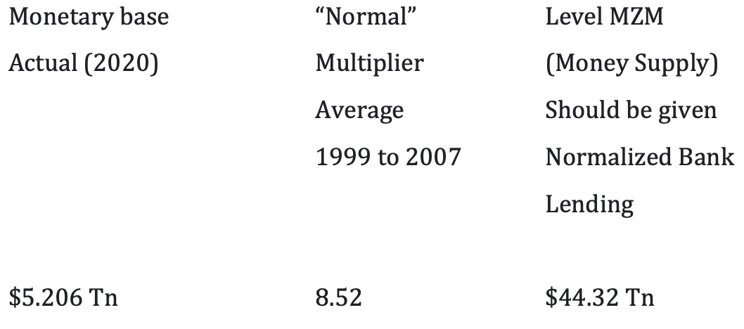
The Total Broad Money Supply (MZM) should be approximately $44.32 tn instead of the current 21.61tn. (If multiplier 2 returns to “normal)
Now, if we adjust the theoretical MZM, to what the nominal GDP should be under normal MZM velocity, then nominal GDP would be.
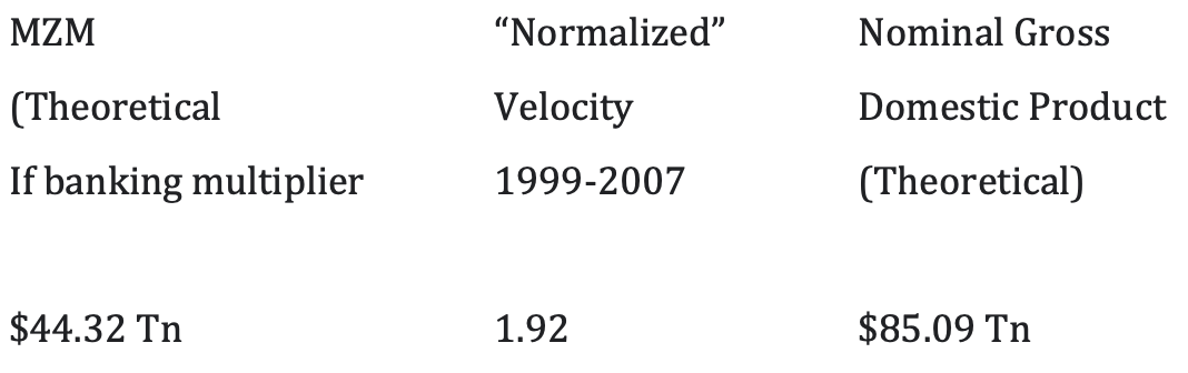
So, if the economy normalizes and returns to the average monetary ratios from the pre-crisis (1999 to 2007) level, then nominal GDP should be approximately $85 tn, instead of the current level of $21.479 tn. Because nominal GDP is made up of “Real (productive) GDP” plus inflation, I contend that the difference between the Theoretical GDP ($85 Tn) and the actual observed GDP ($21.479 Tn) is “Potential Inflation” of ($63.521 TN).
If the economic function returns to normal over say 20 years, price indices should rise by 85/21.479, or 3.96 times. If price levels need to inflate to four times the current level over the next 20 years, the inflation rate would need to average 7 percent over these following 20 years.
The problem with this forecast is, it is too low. It does not take into account extra spending that will be required to keep the economy out of recession. We have a social democracy as our form of government, and the voters will require real economic growth. This will require additional government deficits and most likely further additions to the Federal Reserve balance sheet. The most efficient way of increasing demand in the economy, at a time of recession, is now by growing the Fed balance sheet. We can no longer lower interest rates to spur demand, so it’s fiscal stimulus is the only game left in town.
I think a starting guess, given the need for monetary stimulus, is that The Federal Reserve balance sheet increases required to deal with a recession will be approximately 10 percent of GDP each time, and I think we”ll have two more recessions in the next twenty years, with the monetary base expanding about $2 tn each time. This means the monetary base in our calculation goes from $5.2 tn to $9.2 tn over the following 20 years. Theoretical MZM therefore revises upward from $44.32 tn to $78.38 tn. Therefore, the theoretical inflation expanded GDP is revised from $85 tn to $150 tn. That’s a big number needed for inflation. $150 Nominal GDP future /$ 21.47 current Nominal GDP = 6.98 or prices will then need to go up 7 times to equalize in the economy over the next 20 years. This works out to be approximately 10.25 percent per year inflation average for the next 20 years.
There are many things that can change over the following 20 years. Government policy can be more redistributive, productivity could expand faster than we expect, imported inflation may be more of a problem if costs start rising in countries we import from. All of these concerns would raise the future inflation rate. On the other hand, governments and corporations could strongly move toward cost containment and raise taxes. Both of these would slow the inflation rate, but also harm the economy enough it is unlikely the electorate would continue on this path too long.
This is a scenario very similar to post war Britain and France. In both of these examples, the fiscal deficits appeared to be great. Lower class incomes seemed to magically appear, and domestic demand increased, which flowed through the entire economy. Eventually, this positive outcome was destroyed by the increased inflation, loss of investment, and overall decline in real incomes. This outcome is what I expect for the US in the coming 20 years.
I am not trying to put a political spin on this, wealth distributions have reached maximum historical dispersion. If the economy does not improve lower class incomes, we face an economy with a chronic inability to create domestic demand. We are forced to use fiscal stimulus to get this demand going. The paradox comes in when one considers, many of these same programs will eventually create the inflation that destroys the real incomes of the middle class.